%load ../../rapaio-bootstrap.ipynb
Adding dependency io.github.padreati:rapaio-lib:7.0.1
Solving dependencies
Resolved artifacts count: 1
Add to classpath: /home/ati/work/rapaio-jupyter-kernel/target/mima_cache/io/github/padreati/rapaio-lib/7.0.1/rapaio-lib-7.0.1.jar
Built-in Data sets#
For learning purposes some well-known data sets are already incorporated into rapaio library. All built in data sets are available via rapaio.datasets.Datasets class. This is an utility class which provides some standard data sets used in many statistical and machine learning text books. Some of them are described below
Iris data set#
The Iris flower data set or Fisher’s Iris data set is a multivariate data set introduced by Ronald Fisher in his 1936 paper The use of multiple measurements in taxonomic problems as an example of linear discriminant analysis. It is sometimes called Anderson’s Iris data set because Edgar Anderson collected the data to quantify the morphological variation of Iris flowers of three related species.
Two of the three species were collected in the Gaspé Peninsula all from the same pasture, and picked on the same day and measured at the same time by the same person with the same apparatus.
The data set consists of 50 samples from each of three species of Iris (Iris setosa, Iris virginica and Iris versicolor). There are for measures for each sample: the length and the width of the sepals and petals, in centimeters. Based on the combination of these four features, Fisher developed a linear discriminant model to distinguish the species from each other.
var iris = Datasets.loadIrisDataset();
iris.printSummary();
Frame Summary
=============
* rowCount: 150
* complete: 150/150
* varCount: 5
* varNames:

0. sepal-length : dbl | 3.  petal-width : dbl |
1.  sepal-width : dbl | 4.        class : nom |
2. petal-length : dbl |

* summary:
 sepal-length [dbl]      sepal-width [dbl]      petal-length [dbl]      petal-width [dbl]
       Min. : 4.3000000       Min. : 2.0000000        Min. : 1.0000000       Min. : 0.1000000
    1st Qu. : 5.1000000    1st Qu. : 2.8000000     1st Qu. : 1.6000000    1st Qu. : 0.3000000
     Median : 5.8000000     Median : 3.0000000      Median : 4.3500000     Median : 1.3000000
       Mean : 5.8433333       Mean : 3.0573333        Mean : 3.7580000       Mean : 1.1993333
    2nd Qu. : 6.4000000    2nd Qu. : 3.3000000     2nd Qu. : 5.1000000    2nd Qu. : 1.8000000
       Max. : 7.9000000       Max. : 4.4000000        Max. : 6.9000000       Max. : 2.5000000


       class [nom]
versicolor :    50
    setosa :    50
 virginica :    50
Pearson’s Height Data#
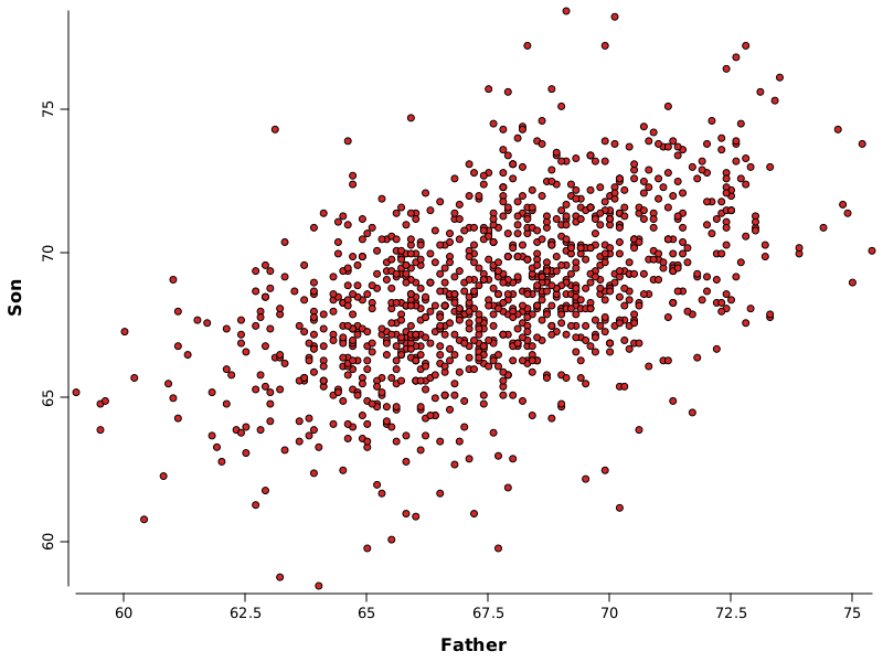
This simple data set comes from a famous experiment by Karl Pearson around 1903. The number of cases is 1078. The original data values were rounded to produce heights to the nearest \(0.1\) inch.
var df = Datasets.loadPearsonHeightDataset();
df.printSummary();
Frame Summary
=============
* rowCount: 1078
* complete: 1078/1078
* varCount: 2
* varNames:

0. Father : dbl |
1.    Son : dbl |

* summary:
   Father [dbl]            Son [dbl]         Mean : 67.6868275    Mean : 68.6842301
   Min. : 59.0000000    Min. : 58.5000000 2nd Qu. : 69.6000000 2nd Qu. : 70.5000000
1st Qu. : 65.8000000 1st Qu. : 66.9000000    Max. : 75.4000000    Max. : 78.4000000
 Median : 67.8000000  Median : 68.6000000
WS.image(points(df.rvar("Father"), df.rvar("Son"), pch.circleFull(), fill(1)));

Advertising data set#
This data set is one of the first data sets used in Introduction to Statistical Learning book to illustrate various topics for linear regression. It contains observations which relates sales as an assumed result of advertising into various types of media communication like TV, radio or newspapers.
var df = Datasets.loadISLAdvertising()
df.printSummary()
Frame Summary
=============
* rowCount: 200
* complete: 200/200
* varCount: 4
* varNames:

0.        TV : dbl |
1.     Radio : dbl |
2. Newspaper : dbl |
3.     Sales : dbl |

* summary:
       TV [dbl]           Radio [dbl]       Newspaper [dbl]           Sales [dbl]
   Min. :   0.7000000    Min. :  0.0000000     Min. :   0.3000000    Min. :  1.6000000
1st Qu. :  74.3750000 1st Qu. :  9.9750000  1st Qu. :  12.7500000 1st Qu. : 10.3750000
 Median : 149.7500000  Median : 22.9000000   Median :  25.7500000  Median : 12.9000000
   Mean : 147.0425000    Mean : 23.2640000     Mean :  30.5540000    Mean : 14.0225000
2nd Qu. : 218.8250000 2nd Qu. : 36.5250000  2nd Qu. :  45.1000000 2nd Qu. : 17.4000000
   Max. : 296.4000000    Max. : 49.6000000     Max. : 114.0000000    Max. : 27.0000000
